Decomposition¶

tICA¶

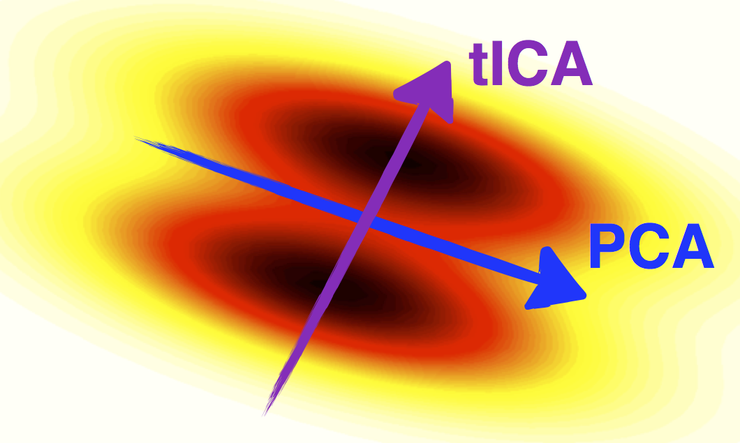
tICA compared to PCA (courtesy of C. R. Schwantes)

Time-structure independent components analysis (tICA) is a method for finding the slowest-relaxing degrees of freedom in a time series data set which can be formed from linear combinations from a set of input degrees of freedom.

tICA can be used as a dimensionality reduction method and, in that capacity, is somewhat similar to PCA. However whereas PCA finds high-variance linear combinations of the input degrees of freedom, tICA finds high-autocorrelation linear combinations of the input degrees of freedom.

The tICA method has one obvious drawback: its solution is a linear combination of all input degrees of freedom, and their relative weights are typically non-zero. This makes each independent component difficult to interpret in an algorithmic fashion because it could comprise hundreds or thousands of different metrics. Because an important property of reaction coordinates is their role in facilitating physical interpretation of the underlying molecular system, we consider it desirable to reduce the number of explicitly used variables. SparseTICA [2] attempts to resolve this interpretability issue by using a sparse approximation to the eigenvalue problem found in tICA and returning independent components composed of only the most relevant degrees of freedom.

Another limitation of tICA is that it is constrained to finding linear correlations between input coordinates. The KernelTICA method [5] provides a natural extension to nonlinear functions by utilizing the kernel trick and represents a substantial improvement in estimating the eigenfunctions of the transfer operator directly.

PCA¶

Principal component analysis (PCA) is a method for finding the most highly varying degrees of freedom in a data set (not necessarily a time series). PCA is useful as a dimensionality reduction method.

Algorithms¶

`tICA`([n_components, lag_time, shrinkage, ...])	Time-structure Independent Component Analysis (tICA)
`SparseTICA`([n_components, lag_time, rho, ...])	Sparse time-structure Independent Component Analysis (tICA).
`PCA`([n_components, copy, whiten, ...])	Principal component analysis (PCA)

Theory¶

PCA¶

PCA tries to find projection vectors that maximize their explained variance, subject to them being uncorrelated and having length one. In the end, these maximal variance projections correspond to the solutions of the following eigenvalue problem:

\[\Sigma v = \lambda v\]

where \(\Sigma\) is the covariance matrix given by:

\[\Sigma_{ij} = \mathbb{E}\Big[ X_i(t) X_j(t) \Big]\]

The problem with using PCA to define a reduced space for biomolecular dynamics, however, is that high-variance degrees of freedom need not be slow (for instance consider a floppy protein tail that varies wildly vs. a single dihedral angle that is required to rotate for a protein to fold). What we really want is to design projections that can best differentiate between slowly equilibrating populations, which is precisely where tICA comes in.

tICA¶

In tICA, the goal is to find projection vectors that maximize their autocorrelation function, subject to them being uncorrelated and having unit variance. It is easy to show [1] that the solution to the tICA problem are the solutions to this generalized eigenvalue problem (which is closely related to the PCA eigenvalue problem):

\[C^{(\Delta t)} v = \lambda \Sigma v\]

where \(C^{(\Delta t)}\) is the time lag correlation matrix defined by:

\[C^{(\Delta t)}_{ij} = \mathbb{E}\Big[ X_i(t) X_j(t+\Delta t) \Big]\]

Given this solution, we can use the tICA method to define a reduced dimensionality representation of each \(\mathbf{X}(t)\) by projecting the vector onto the slowest \(n\) tICs.

Hyperparameters¶

There are two parameters introduced in the tICA method. The first is \(\Delta t\), which is used in the calculation of the time-lag correlation matrix (\(C^{(\Delta t)}\)). The second is \(n\), which is the number of tICs to project onto when calculating distances between conformations. You can use the GMRQ score to choose these parameters. Typical values are of order nanoseconds and tens, respectively.

Drawbacks¶

Since part of the process of using tICA is a dimensionality reduction, there is always the opportunity to throw out important pieces of information. By throwing out the faster degrees of freedom, we can better estimate the slowest timescales; but this comes with the trade-off of not representing the fast timescales correctly.

Combination with MSM¶

While the tICs are themselves approximations to the dominant eigenfunctions of the propagator / transfer operator, the approach taken in [1] and [2] is to “stack” tICA with MSMs. For example, in [2], Perez-Hernandez et al. first measured the 66 atom-atom distances between a set of atoms in each frame of their MD trajectories, and then used tICA to find the slowest 1, 4, and 10 linear combinations of these degrees of freedom and transform the 66-dimensional dataset into a 1, 4, or 10-dimensional dataset. Then, they applied KMeans to the resulting data and built an MSM.

References¶

[1]	(1, 2) Schwantes, Christian R., and Vijay S. Pande. Improvements in Markov State Model Construction Reveal Many Non-Native Interactions in the Folding of NTL9 J. Chem Theory Comput. 9.4 (2013): 2000-2009.

[2]	(1, 2, 3) Perez-Hernandez, Guillermo, et al. Identification of slow molecular order parameters for Markov model construction J Chem. Phys (2013): 015102.

[3]	Naritomi, Yusuke, and Sotaro Fuchigami. Slow dynamics in protein fluctuations revealed by time-structure based independent component analysis: The case of domain motions J. Chem. Phys. 134.6 (2011): 065101.

[4]	McGibbon, R. T. & Pande, V. S. Identification of simple reaction coordinates from complex dynamics ArXiv 16 (2016).

[5]	Schwantes, Christian R., and Vijay S. Pande. Modeling Molecular Kinetics with tICA and the Kernel Trick J. Chem Theory Comput. 11.2 (2015): 600–608.