Hidden Markov models (HMMs)
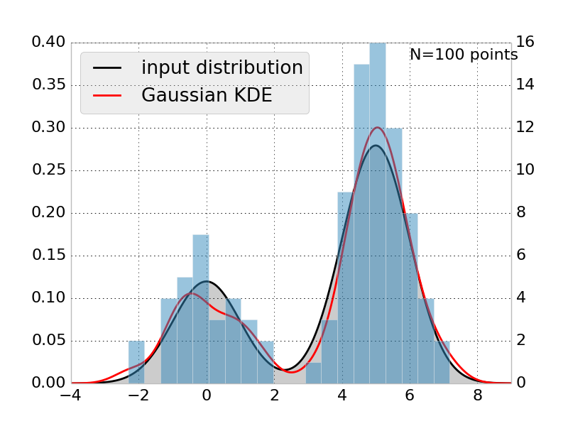
Comparison of histogram and KDE for a 1D PDF.
Background
One potential weakness of of MSMs is that they use states discrete states with “hard” cutoffs. In some sense, an MSM forms an approximation to the transfer operator in the same sense that a histogram is an approximation a probability density function. When a probability density function is smooth, better performance can often be achieved with kernel density estimators, or mixture models, which smooth the data in a potentially more natural way.
A Gaussian hidden Markov model (HMM) is one way of applying this same logic to probabilistic models of the dynamics of molecular system. Like MSMs, the HMM also models the dynamics of the system as a 1st order Markov jump process between discrete set of states. The difference is that the states in the HMM are not associated with discrete non-overlapping regions of phase space defined by clustering – instead the states are Gaussian distributions. Because the Gaussian distribution has infinite support, there is no unique and unambiguous mapping from conformation to state. Each state is a distribution over all conformations.
HMMs have been widely used in many many fields, from speech processing to bioinformatics. Many good reviews have been written, such as [1].
L1-Regularized Reversible Gaussian HMM
In [2], McGibbon et. al. introduced a reversible Gaussian HMM for studying protein dynamics. The class GaussianFusionHMM implements the algorithm described in that paper. Compared to a “vanilla” HMM, it has a couple bells and whistles.
- The transition matrix is constrained to obey detailed balance. Detailed balance is a necessary condition for the the model to satisfy the 2nd law of thermodynamics. It also aids analysis, because models that don’t satisfy detailed balance don’t necessarily have a unique equilibrium distribution that they relax to in the limit of infinite time.
- We added a penalty term (tunable via the fusion_prior hyperparameter) on the pairwise difference between the means of each of the states. This helps encourage a sense of sparisty where each state might be different from the other states along only a subset of the coordinates.
The implementation is also quite fast. There is a backend for NVIDIA GPUs in CUDA as well as a multithreaded and explicitly vectorized CPU implementation. Compared to a default implementation, it can be ~10x-100x faster.
Algorithms
| GaussianFusionHMM(n_states, n_features[, ...]) | Reversible Gaussian Hidden Markov Model L1-Fusion Regularization |
| VonMisesHMM([n_states, transmat, ...]) | Hidden Markov Model with von Mises Emissions |
Example
from msmbuilder.featurizer import SuperposeFeaturizer
from msmbuilder.ghmm import GaussianFusionHMM

xtal = md.load('crystal-structure.pdb')
alpha_carbons = [a.index for a in xtal.topology.atoms if a.name == 'CA']
f = SuperposeFeaturizer(alpha_carbons, xtal)

dataset = []
for trajectory_file in ['trj0.xtc', 'trj1.xtc']:
    t = md.load(trajectory_file, top=xtal)
    dataset.append(f.partial_transform(t))

hmm = GaussianFusionHMM(n_states=8, n_features=len(alpha_carbons))
hmm.fit(dataset)
print hmm.timescales_()
References
| [1] | Rabiner, Lawrence, and Biing-Hwang Juang. An introduction to hidden Markov models ASSP Magazine, IEEE 3.1 (1986): 4-16. |
| [2] | McGibbon, Robert T. et al., Understanding Protein Dynamics with L1-Regularized Reversible Hidden Markov Models Proc. 31st Intl. Conf. on Machine Learning (ICML). 2014. |