Fs Peptide (command line)
Modeling dynamics of FS Peptide
This example shows a typical, basic usage of the MSMBuilder command line to model dynamics of a protein system.
# Work in a temporary directory
import tempfile
import os
os.chdir(tempfile.mkdtemp())
# Since this is running from an IPython notebook,
# we prefix all our commands with "!"
# When running on the command line, omit the leading "!"
! msmb -h
Get example data
! msmb FsPeptide --data_home ./
! tree
Featurization
The raw (x, y, z) coordinates from the simulation do not respect the translational and rotational symmetry of our problem. A Featurizer transforms cartesian coordinates into other representations. Here we use the DihedralFeaturizer to turn our data into phi and psi dihedral angles. Observe that the 264*3-dimensional space is reduced to 84 dimensions.
# Remember '\' is the line-continuation marker
# You can enter this command on one line
! msmb DihedralFeaturizer \
    --out featurizer.pkl  \
    --transformed diheds  \
    --top fs_peptide/fs-peptide.pdb \
    --trjs "fs_peptide/*.xtc" \
    --stride 10
Preprocessing
Since the range of values in our raw data can vary widely from feature to feature, we can scale values to reduce bias. Here we use the RobustScaler to center and scale our dihedral angles by their respective interquartile ranges.
! msmb RobustScaler \
    -i diheds \
    --transformed scaled_diheds.h5
Intermediate kinetic model: tICA
tICA is similar to principal component analysis (see "tICA vs. PCA" example). Note that the 84-dimensional space is reduced to 4 dimensions.
! msmb tICA -i scaled_diheds.h5 \
    --out tica_model.pkl \
    --transformed tica_trajs.h5 \
    --n_components 4 \
    --lag_time 2
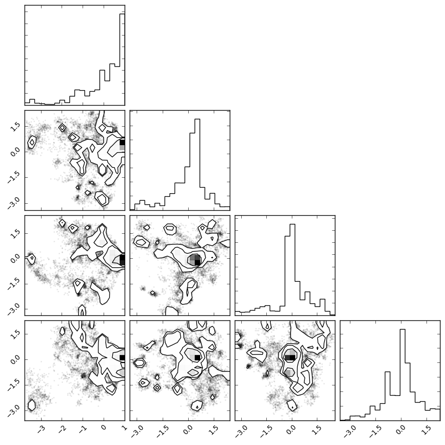
tICA Histogram
We can histogram our data projecting along the two slowest degrees of freedom (as found by tICA). You have to do this in a python script.
from msmbuilder.dataset import dataset
ds = dataset('tica_trajs.h5')

%matplotlib inline
import msmexplorer as msme
import numpy as np
txx = np.concatenate(ds)
_ = msme.plot_histogram(txx)
Clustering
Conformations need to be clustered into states (sometimes written as microstates). We cluster based on the tICA projections to group conformations that interconvert rapidly. Note that we transform our trajectories from the 4-dimensional tICA space into a 1-dimensional cluster index.
! msmb MiniBatchKMeans -i tica_trajs.h5 \
    --transformed labeled_trajs.h5 \
    --out clusterer.pkl \
    --n_clusters 100 \
    --random_state 42
MSM
We can construct an MSM from the labeled trajectories
! msmb MarkovStateModel -i labeled_trajs.h5 \
    --out msm.pkl \
    --lag_time 2
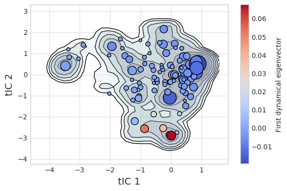
Plot Free Energy Landscape
Subsequent plotting and analysis should be done from Python
from msmbuilder.utils import load
msm = load('msm.pkl')
clusterer = load('clusterer.pkl')

assignments = clusterer.partial_transform(txx)
assignments = msm.partial_transform(assignments)

from matplotlib import pyplot as plt
msme.plot_free_energy(txx, obs=(0, 1), n_samples=10000,
                      pi=msm.populations_[assignments],
                      xlabel='tIC 1', ylabel='tIC 2')
plt.scatter(clusterer.cluster_centers_[msm.state_labels_, 0],
            clusterer.cluster_centers_[msm.state_labels_, 1],
            s=1e4 * msm.populations_,       # size by population
            c=msm.left_eigenvectors_[:, 1], # color by eigenvector
            cmap="coolwarm",
            zorder=3
           )
plt.colorbar(label='First dynamical eigenvector')
plt.tight_layout()
(Fs-Peptide-command-line.ipynb; Fs-Peptide-command-line.eval.ipynb; Fs-Peptide-command-line.py)