Fs Peptide¶

Modeling dynamics of FS Peptide¶

This example shows a typical, basic usage of the MSMExplorer command line to plot the modeled dynamics of a protein system.

In [1]:

%matplotlib inline

from msmbuilder.featurizer import DihedralFeaturizer
from msmbuilder.decomposition import tICA
from msmbuilder.preprocessing import RobustScaler
from msmbuilder.cluster import MiniBatchKMeans
from msmbuilder.msm import MarkovStateModel

import numpy as np

import msmexplorer as msme
from msmexplorer.example_datasets import FsPeptide

rs = np.random.RandomState(42)

/home/travis/miniconda3/envs/docenv/lib/python3.5/site-packages/matplotlib/font_manager.py:273: UserWarning: Matplotlib is building the font cache using fc-list. This may take a moment.
  warnings.warn('Matplotlib is building the font cache using fc-list. This may take a moment.')
/home/travis/miniconda3/envs/docenv/lib/python3.5/site-packages/matplotlib/font_manager.py:273: UserWarning: Matplotlib is building the font cache using fc-list. This may take a moment.
  warnings.warn('Matplotlib is building the font cache using fc-list. This may take a moment.')

Load Fs Peptide Data¶

In [2]:

trajs = FsPeptide(verbose=False).get().trajectories

/home/travis/miniconda3/envs/docenv/lib/python3.5/site-packages/mdtraj/formats/pdb/pdbfile.py:196: UserWarning: Unlikely unit cell vectors detected in PDB file likely resulting from a dummy CRYST1 record. Discarding unit cell vectors.
  warnings.warn('Unlikely unit cell vectors detected in PDB file likely '

Extract Backbone Dihedrals¶

The raw (x, y, z) coordinates from the simulation do not respect the translational and rotational symmetry of our problem. A Featurizer transforms cartesian coordinates into other representations. Here we use the DihedralFeaturizer to turn our data into phi and psi dihedral angles. Observe that the 264*3-dimensional space is reduced to 84 dimensions.

In [3]:

featurizer = DihedralFeaturizer(types=['phi', 'psi'])
diheds = featurizer.fit_transform(trajs)

Preprocess Data¶

RobustScaler removes the median and scales the data according to the Interquartile Range (IQR). The IQR is the range between the 1st quartile (25th quantile) and the 3rd quartile (75th quantile).

In [4]:

scaler = RobustScaler()
scaled_data = scaler.fit_transform(diheds)

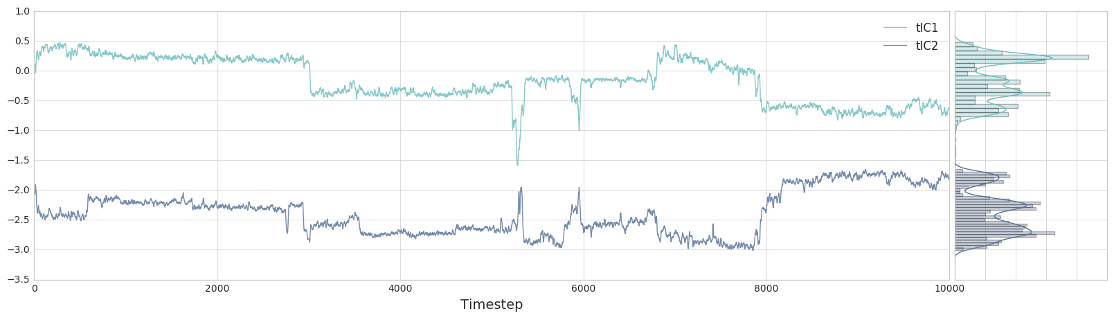
Perform Dimensionality Reduction¶

tICA is similar to principal component analysis (see "tICA vs. PCA" example). Note that the 84-dimensional space is reduced to 2 dimensions.

In [5]:

tica_model = tICA(lag_time=10, n_components=2, kinetic_mapping=True)
tica_trajs = tica_model.fit_transform(scaled_data)

ax, side_ax = msme.plot_trace(tica_trajs[0][:, 0], window=10,
                              label='tIC1', xlabel='Timestep')
_ = msme.plot_trace(tica_trajs[0][:, 1], window=10, label='tIC2',
                    xlabel='Timestep', color='rawdenim', ax=ax,
                    side_ax=side_ax)

/home/travis/miniconda3/envs/docenv/lib/python3.5/site-packages/statsmodels/nonparametric/kdetools.py:20: VisibleDeprecationWarning: using a non-integer number instead of an integer will result in an error in the future
  y = X[:m/2+1] + np.r_[0,X[m/2+1:],0]*1j

Perform Clustering¶

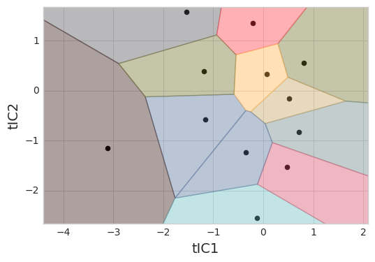
Conformations need to be clustered into states (sometimes written as microstates). We cluster based on the tICA projections to group conformations that interconvert rapidly. Note that we transform our trajectories from the 4-dimensional tICA space into a 1-dimensional cluster index.

In [6]:

clusterer = MiniBatchKMeans(n_clusters=12, random_state=rs)
clustered_trajs = clusterer.fit_transform(tica_trajs)

_ = msme.plot_voronoi(clusterer, xlabel='tIC1', ylabel='tIC2')

Construct MSM¶

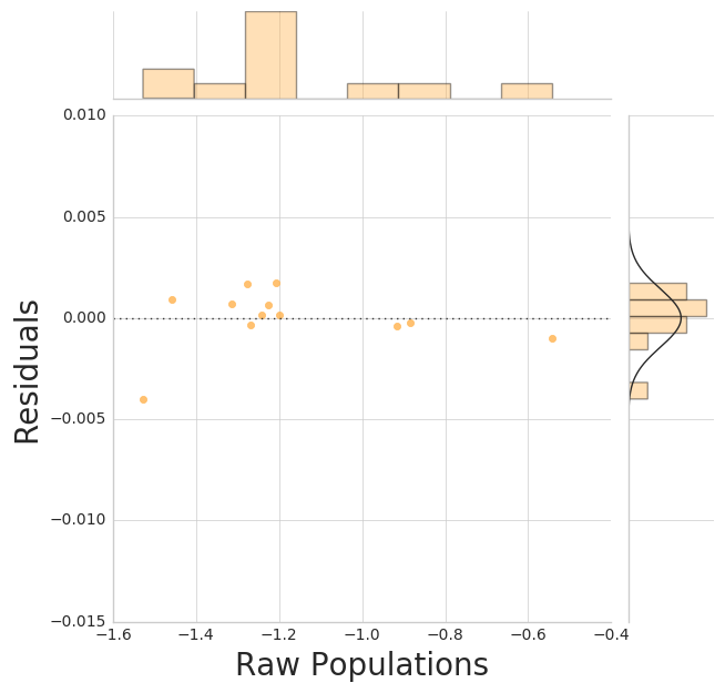
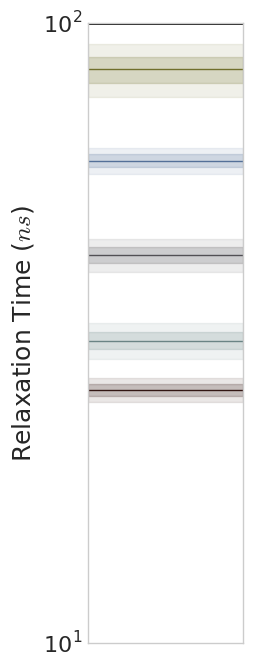
We can construct an MSM from the labeled trajectories and plot the implied timescales.

In [7]:

msm = MarkovStateModel(lag_time=1, n_timescales=5)
assigns = msm.fit_transform(clustered_trajs)

_ = msme.plot_pop_resids(msm, color='tarragon')

MSM contains 1 strongly connected component above weight=1.00. Component 0 selected, with population 100.000000%

In [8]:

_ = msme.plot_timescales(msm, ylabel=r'Relaxation Time ($ns$)')

Free Energy Landscape¶

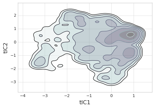
From our MSM and tICA data, we can construct a 2-D free energy landscape.

In [9]:

data = np.concatenate(tica_trajs, axis=0)
pi_0 = msm.populations_[np.concatenate(assigns, axis=0)]

_ = msme.plot_free_energy(data, obs=(0, 1), n_samples=10000,
                          pi=pi_0, gridsize=100, vmax=5.,
                          n_levels=8, cut=5, xlabel='tIC1',
                          ylabel='tIC2', random_state=rs)

(Fs-Peptide-Example.ipynb; Fs-Peptide-Example.eval.ipynb; Fs-Peptide-Example.py)