Fs Peptide (using dataset)
Modeling dynamics of FS Peptide
This example shows a typical, basic usage of MSMBuilder to model dynamics of a protein system.
MSMBuilder includes example datasets
The following cell downloads an example protein dataset or uses the data provided by the msmb_data conda package. In practice, you will generate your own dataset by running molecular dynamics (MD) on your system of interest. MSMBuilder does not run MD.
# Download example dataset
from msmbuilder.example_datasets import FsPeptide
fs_peptide = FsPeptide(verbose=False)
fs_peptide.cache()
# Work in a temporary directory
import tempfile
import os
os.chdir(tempfile.mkdtemp())
The dataset object
MD datasets are usually quite large. It doesn't make sense to load everything into memory at once. The dataset object lazily-loads trajectories as they are needed. Below, we create a dataset out of the 28 *.xtc files we downloaded above. Since the data was saved at 50 ps / frame, we only load every 10th frame (with a new frequency of 0.5/ns).
from msmbuilder.dataset import dataset
xyz = dataset(fs_peptide.data_dir + "/*.xtc",
              topology=fs_peptide.data_dir + '/fs-peptide.pdb',
              stride=10)
print("{} trajectories".format(len(xyz)))
# msmbuilder does not keep track of units! You must keep track of your
# data's timestep
to_ns = 0.5
print("with length {} ns".format(set(len(x)*to_ns for x in xyz)))
Featurization
The raw (x, y, z) coordinates from the simulation do not respect the translational and rotational symmetry of our problem. A Featurizer transforms cartesian coordinates into other representations. Here we use the DihedralFeaturizer to turn our data into phi and psi dihedral angles. Observe that the 264*3-dimensional space is reduced to 84 dimensions
from msmbuilder.featurizer import DihedralFeaturizer
featurizer = DihedralFeaturizer(types=['phi', 'psi'])
diheds = xyz.fit_transform_with(featurizer, 'diheds/', fmt='dir-npy')

print(xyz[0].xyz.shape)
print(diheds[0].shape)
Preprocessing
Since the range of values in our raw data can vary widely from feature to feature, we can scale values to reduce bias. Here we use the RobustScaler to center and scale our dihedral angles by their respective interquartile ranges.
from msmbuilder.preprocessing import RobustScaler
scaler = RobustScaler()
scaled_diheds = diheds.fit_transform_with(scaler, 'scaled_diheds/', fmt='dir-npy')

print(diheds[0].shape)
print(scaled_diheds[0].shape)
Intermediate kinetic model: tICA
tICA is similar to principal component analysis (see "tICA vs. PCA" example). Note that the 84-dimensional space is reduced to 4 dimensions.
from msmbuilder.decomposition import tICA
tica_model = tICA(lag_time=2, n_components=4)
# fit and transform can be done in seperate steps:
tica_model = scaled_diheds.fit_with(tica_model)
tica_trajs = scaled_diheds.transform_with(tica_model, 'ticas/', fmt='dir-npy')

print(diheds[0].shape)
print(tica_trajs[0].shape)
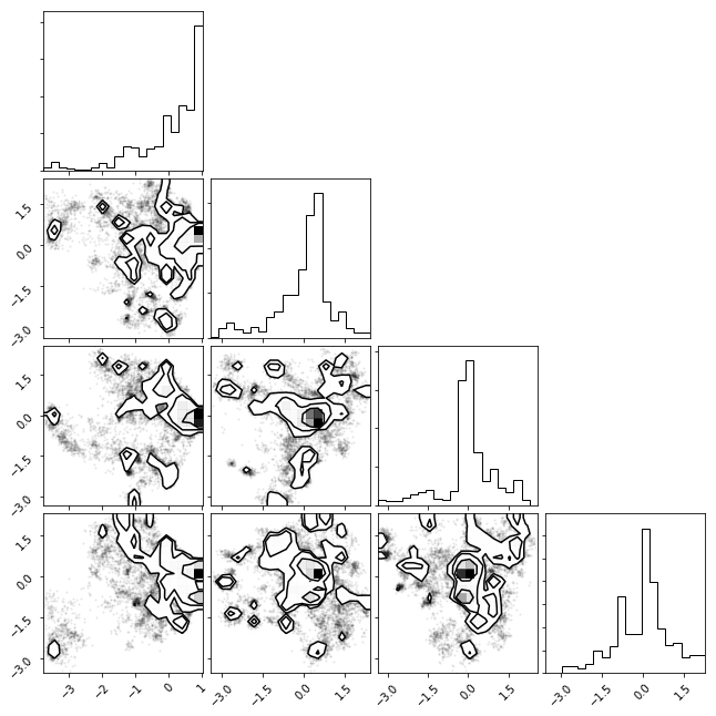
tICA Histogram
We can histogram our data projecting along the two slowest degrees of freedom (as found by tICA)
%matplotlib inline
import msmexplorer as msme
import numpy as np
txx = np.concatenate(tica_trajs)
_ = msme.plot_histogram(txx)
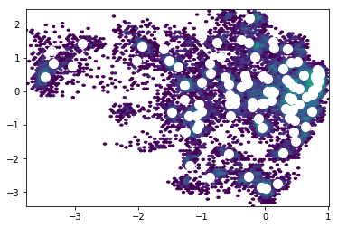
Clustering
Conformations need to be clustered into states (sometimes written as microstates). We cluster based on the tICA projections to group conformations that interconvert rapidly. Note that we transform our trajectories from the 4-dimensional tICA space into a 1-dimensional cluster index.
from msmbuilder.cluster import MiniBatchKMeans
clusterer = MiniBatchKMeans(n_clusters=100, random_state=42)
clustered_trajs = tica_trajs.fit_transform_with(
    clusterer, 'kmeans/', fmt='dir-npy'
)

print(tica_trajs[0].shape)
print(clustered_trajs[0].shape)
from matplotlib import pyplot as plt
plt.hexbin(txx[:,0], txx[:,1], bins='log', mincnt=1, cmap='viridis')
plt.scatter(clusterer.cluster_centers_[:,0],
            clusterer.cluster_centers_[:,1],
            s=100, c='w')
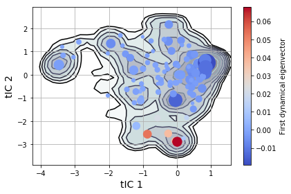
MSM
We can construct an MSM from the labeled trajectories
from msmbuilder.msm import MarkovStateModel
from msmbuilder.utils import dump
msm = MarkovStateModel(lag_time=2, n_timescales=20)
msm.fit(clustered_trajs)
assignments = clusterer.partial_transform(txx)
assignments = msm.partial_transform(assignments)
msme.plot_free_energy(txx, obs=(0, 1), n_samples=10000,
                      pi=msm.populations_[assignments],
                      xlabel='tIC 1', ylabel='tIC 2')
plt.scatter(clusterer.cluster_centers_[msm.state_labels_, 0],
            clusterer.cluster_centers_[msm.state_labels_, 1],
            s=1e4 * msm.populations_,       # size by population
            c=msm.left_eigenvectors_[:, 1], # color by eigenvector
            cmap="coolwarm",
            zorder=3)
plt.colorbar(label='First dynamical eigenvector')
plt.tight_layout()
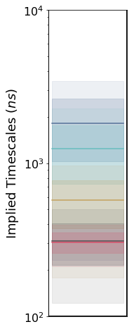
msm.timescales_
msme.plot_timescales(msm, n_timescales=5,
                     ylabel='Implied Timescales ($ns$)')
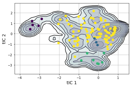
Macrostate Model
from msmbuilder.lumping import PCCAPlus
pcca = PCCAPlus.from_msm(msm, n_macrostates=4)
macro_trajs = pcca.transform(clustered_trajs)
msme.plot_free_energy(txx, obs=(0, 1), n_samples=10000,
                      pi=msm.populations_[assignments],
                      xlabel='tIC 1', ylabel='tIC 2')
plt.scatter(clusterer.cluster_centers_[msm.state_labels_, 0],
            clusterer.cluster_centers_[msm.state_labels_, 1],
            s=50,
            c=pcca.microstate_mapping_,
            zorder=3
           )
plt.tight_layout()
(Fs-Peptide-with-dataset.ipynb; Fs-Peptide-with-dataset.eval.ipynb; Fs-Peptide-with-dataset.py)