tICA vs. PCA¶

This example uses OpenMM to generate example data to compare two methods for dimensionality reduction: tICA and PCA.

Define dynamics¶

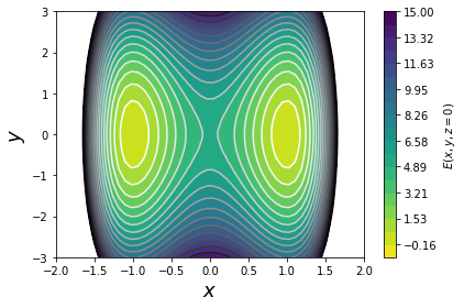
First, let's use OpenMM to run some dynamics on the 3D potential energy function

$$E(x,y,z) = 5 \cdot (x-1)^2 \cdot (x+1)^2 + y^2 + z^2$$

From looking at this equation, we can see that along the x dimension, the potential is a double-well, whereas along the y and z dimensions, we've just got a harmonic potential. So, we should expect that x is the slow degree of freedom, whereas the system should equilibrate rapidly along y and z.

In [1]:

%matplotlib inline
import numpy as np
from matplotlib import pyplot as plt

xx, yy = np.meshgrid(np.linspace(-2,2), np.linspace(-3,3))
zz = 0 # We can only visualize so many dimensions
ww = 5 * (xx-1)**2 * (xx+1)**2 + yy**2 + zz**2
c = plt.contourf(xx, yy, ww, np.linspace(-1, 15, 20), cmap='viridis_r')
plt.contour(xx, yy, ww, np.linspace(-1, 15, 20), cmap='Greys')
plt.xlabel('$x$', fontsize=18)
plt.ylabel('$y$', fontsize=18)
plt.colorbar(c, label='$E(x, y, z=0)$')
plt.tight_layout()

In [2]:

import simtk.openmm as mm
def propagate(n_steps=10000):
    system = mm.System()
    system.addParticle(1)
    force = mm.CustomExternalForce('5*(x-1)^2*(x+1)^2 + y^2 + z^2')
    force.addParticle(0, [])
    system.addForce(force)
    integrator = mm.LangevinIntegrator(500, 1, 0.02)
    context = mm.Context(system, integrator)
    context.setPositions([[0, 0, 0]])
    context.setVelocitiesToTemperature(500)
    x = np.zeros((n_steps, 3))
    for i in range(n_steps):
        x[i] = (context.getState(getPositions=True)
                .getPositions(asNumpy=True)
                ._value)
        integrator.step(1)
    return x

Run Dynamics¶

Okay, let's run the dynamics. The first plot below shows the x, y and z coordinate vs. time for the trajectory, and the second plot shows each of the 1D and 2D marginal distributions.

In [3]:

trajectory = propagate(10000)

ylabels = ['x', 'y', 'z']
for i in range(3):
    plt.subplot(3, 1, i+1)
    plt.plot(trajectory[:, i])
    plt.ylabel(ylabels[i])
plt.xlabel('Simulation time')
plt.tight_layout()

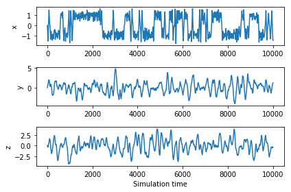
Note that the variance of x is much lower than the variance in y or z, despite its bi-modal distribution.

Fit tICA and PCA models¶

In [4]:

from msmbuilder.decomposition import tICA, PCA
tica = tICA(n_components=1, lag_time=100)
pca = PCA(n_components=1)
tica.fit([trajectory])
pca.fit([trajectory])

/home/travis/miniconda3/envs/docenv/lib/python3.6/site-packages/sklearn/cross_validation.py:41: DeprecationWarning: This module was deprecated in version 0.18 in favor of the model_selection module into which all the refactored classes and functions are moved. Also note that the interface of the new CV iterators are different from that of this module. This module will be removed in 0.20.
  "This module will be removed in 0.20.", DeprecationWarning)
/home/travis/miniconda3/envs/docenv/lib/python3.6/site-packages/sklearn/grid_search.py:42: DeprecationWarning: This module was deprecated in version 0.18 in favor of the model_selection module into which all the refactored classes and functions are moved. This module will be removed in 0.20.
  DeprecationWarning)

Out[4]:

PCA(copy=True, iterated_power='auto', n_components=1, random_state=None,
  svd_solver='auto', tol=0.0, whiten=False)

See what they find¶

In [5]:

plt.subplot(1,2,1)
plt.title('1st tIC')
plt.bar([1,2,3], tica.components_[0], color='b')
plt.xticks([1.5,2.5,3.5], ['x', 'y', 'z'])
plt.subplot(1,2,2)
plt.title('1st PC')
plt.bar([1,2,3], pca.components_[0], color='r')
plt.xticks([1.5,2.5,3.5], ['x', 'y', 'z'])
plt.show()

print('1st tIC', tica.components_ / np.linalg.norm(tica.components_))
print('1st PC ', pca.components_ / np.linalg.norm(pca.components_))

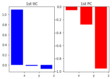
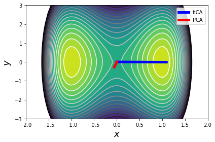
1st tIC [[ 0.99767417 -0.0116976  -0.06715221]]
1st PC  [[-0.05327395 -0.27673402 -0.95946869]]

Note that the first tIC "finds" a projection that just resolves the x coordinate, whereas PCA doesn't.

In [6]:

c = plt.contourf(xx, yy, ww, np.linspace(-1, 15, 20), cmap='viridis_r')
plt.contour(xx, yy, ww, np.linspace(-1, 15, 20), cmap='Greys')

plt.plot([0, tica.components_[0, 0]],
         [0, tica.components_[0, 1]],
         lw=5, color='b', label='tICA')

plt.plot([0, pca.components_[0, 0]],
         [0, pca.components_[0, 1]],
         lw=5, color='r', label='PCA')

plt.xlabel('$x$', fontsize=18)
plt.ylabel('$y$', fontsize=18)
plt.legend(loc='best')
plt.tight_layout()

(tICA-vs-PCA.ipynb; tICA-vs-PCA.eval.ipynb; tICA-vs-PCA.py)