GMRQ Model Selection
GMRQ Model Selection
We use cross-validation and the generalized matrix Rayleigh quotient (GMRQ) for selecting MSM hyperparameters. The GMRQ is a criterion which "scores" how well the MSM eigenvectors generated on the training dataset serve as slow coordinates for the test dataset [1].
[1] McGibbon, R. T. and V. S. Pande, Variational cross-validation of slow dynamical modes in molecular kinetics (2014)
Get Data
This example uses the doublewell dataset, which consists of ten trajectories in 1D with $x \in [-\pi, \pi]$.
from msmbuilder.example_datasets import DoubleWell
trajectories = DoubleWell(random_state=0).get().trajectories
# sub-sample by taking only every 100th data point in each trajectory.
trajectories = [t[::100] for t in trajectories]
print([t.shape for t in trajectories])
Set up pipeline
The Pipeline is a way of connecting together multiple estimators, so that we can create a custom model that
performs a sequence of steps. This model is relatively simple. It will first discretize the trajectory data
onto an evenly spaced grid between $-\pi$ and $\pi$, and then build an MSM.
from sklearn.pipeline import Pipeline
from msmbuilder.cluster import NDGrid
from msmbuilder.msm import MarkovStateModel
import numpy as np

model = Pipeline([
    ('grid', NDGrid(min=-np.pi, max=np.pi)),
    ('msm', MarkovStateModel(n_timescales=1, lag_time=1, reversible_type='transpose', verbose=False))
])
Cross validation
To get an accurate indication of how well our MSMs are doing at finding the dominant eigenfunctions of our stochastic process, we need to consider the tendency of statistical models to overfit their training data. Our MSMs might build transition matrices which fit the noise in training data as opposed to the underlying signal. One way to combat overfitting in a data-efficient way is with cross validation. This example uses 5-fold cross validation.
from sklearn.cross_validation import KFold
n_states = [5, 10, 25, 50, 100, 200, 500, 750]
cv = KFold(len(trajectories), n_folds=5)
results = []

for n in n_states:
    model.set_params(grid__n_bins_per_feature=n)
    for fold, (train_index, test_index) in enumerate(cv):
        train_data = [trajectories[i] for i in train_index]
        test_data = [trajectories[i] for i in test_index]

        # fit model with a subset of the data (training data).
        # then we'll score it on both this training data (which
        # will give an overly-rosy picture of its performance)
        # and on the test data.
        model.fit(train_data)
        train_score = model.score(train_data)
        test_score = model.score(test_data)

        results.append({
            'train_score': train_score,
            'test_score': test_score,
            'n_states': n,
            'fold': fold})
Use pandas to query our data
import pandas as pd
results = pd.DataFrame(results)
results.head()
Find the average for each fold
We use the median for its tolerance to outliers. Mean works too.
avgs = (results
         .groupby('n_states')
         .aggregate(np.median)
         .drop('fold', axis=1))
avgs
best_n = avgs['test_score'].argmax()
best_score = avgs.loc[best_n, 'test_score']
print(best_n, "states gives the best score:", best_score)
Plot
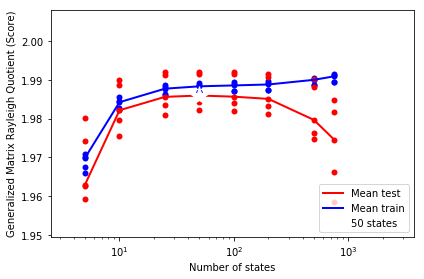
This plot is very similar to figure 1 from McGibbon and Pande. It shows that the performance on the training set keeps going up as we increase the number of states (with the amount of data fixed), whereas the test performance peaks and then starts going down.
We should pick the model with the highest average test set performance. In this example, we're only choosing over the number of MSMs states, but this method can also be used to evaluate the clustering method and any pre-processing like tICA.
However, you do need to fix the number of dynamical processes to "score" (this is the n_timescales attribute for MarkovStateModel), as well as the lag time.
%matplotlib inline
from matplotlib import pyplot as plt

plt.scatter(results['n_states'], results['train_score'], c='b', lw=0, label=None)
plt.scatter(results['n_states'], results['test_score'],  c='r', lw=0, label=None)

plt.plot(avgs.index, avgs['test_score'], c='r', lw=2, label='Mean test')
plt.plot(avgs.index, avgs['train_score'], c='b', lw=2, label='Mean train')

plt.plot(best_n, best_score, c='w',
         marker='*', ms=20, label='{} states'.format(best_n))

plt.xscale('log')
plt.xlim((min(n_states)*.5, max(n_states)*5))
plt.ylabel('Generalized Matrix Rayleigh Quotient (Score)')
plt.xlabel('Number of states')

plt.legend(loc='lower right', numpoints=1)
plt.tight_layout()
(GMRQ-Model-Selection.ipynb; GMRQ-Model-Selection.eval.ipynb; GMRQ-Model-Selection.py)