Two dimensional trace plot¶

from msmbuilder.example_datasets import FsPeptide
from msmbuilder.featurizer import DihedralFeaturizer
from msmbuilder.decomposition import tICA
from msmbuilder.cluster import MiniBatchKMeans
from msmbuilder.msm import MarkovStateModel
from matplotlib import pyplot as pp
import numpy as np

import msmexplorer as msme

rs = np.random.RandomState(42)

# Load Fs Peptide Data
trajs = FsPeptide().get().trajectories

# Extract Backbone Dihedrals
featurizer = DihedralFeaturizer(types=['phi', 'psi'])
diheds = featurizer.fit_transform(trajs)

# Perform Dimensionality Reduction
tica_model = tICA(lag_time=2, n_components=2)
tica_trajs = tica_model.fit_transform(diheds)

# Plot free 2D free energy (optional)
txx = np.concatenate(tica_trajs, axis=0)
ax = msme.plot_free_energy(
    txx, obs=(0, 1), n_samples=100000,
    random_state=rs,
    shade=True,
    clabel=True,
    clabel_kwargs={'fmt': '%.1f'},
    cbar=True,
    cbar_kwargs={'format': '%.1f', 'label': 'Free energy (kcal/mol)'}
)
# Now plot the first trajectory on top of it to inspect it's movement
msme.plot_trace2d(
    data=tica_trajs[0], ts=0.2, ax=ax,
    scatter_kwargs={'s': 2},
    cbar_kwargs={'format': '%d', 'label': 'Time (ns)',
                 'orientation': 'horizontal'},
    xlabel='tIC 1', ylabel='tIC 2'
)
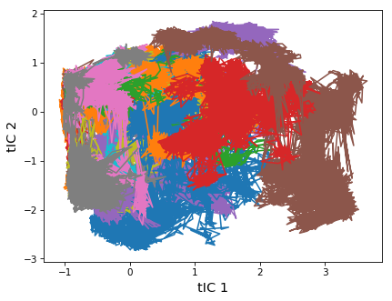
# Finally, let's plot every trajectory to see the individual sampled regions
f, ax = pp.subplots()
msme.plot_trace2d(tica_trajs, ax=ax, xlabel='tIC 1', ylabel='tIC 2')
pp.show()