This example shows a typical, basic usage of the MSMExplorer command line to plot the modeled dynamics of a protein system.
%matplotlib inline

from msmbuilder.example_datasets import FsPeptide
from msmbuilder.featurizer import DihedralFeaturizer
from msmbuilder.decomposition import tICA
from msmbuilder.preprocessing import RobustScaler
from msmbuilder.cluster import MiniBatchKMeans
from msmbuilder.msm import MarkovStateModel

import numpy as np

import msmexplorer as msme

rs = np.random.RandomState(42)
This dataset consists of 28 molecular dynamics trajectories of Fs peptide (Ace-A_5(AAARA)_3A-NME), a widely studied model system for protein folding.
Each trajectory is 500 ns in length, and saved at a 50 ps time interval (14 $\mu$s aggegrate sampling)
trajs = FsPeptide(verbose=False).get().trajectories
The raw (x, y, z) coordinates from the simulation do not respect the translational and rotational symmetry of our problem. A Featurizer transforms cartesian coordinates into other representations. Here we use the DihedralFeaturizer to turn our data into phi and psi dihedral angles. Observe that the 264*3-dimensional space is reduced to 84 dimensions.
featurizer = DihedralFeaturizer(types=['phi', 'psi'])
diheds = featurizer.fit_transform(trajs)
RobustScaler removes the median and scales the data according to the Interquartile Range (IQR). The IQR is the range between the 1st quartile (25th quantile) and the 3rd quartile (75th quantile).
scaler = RobustScaler()
scaled_data = scaler.fit_transform(diheds)
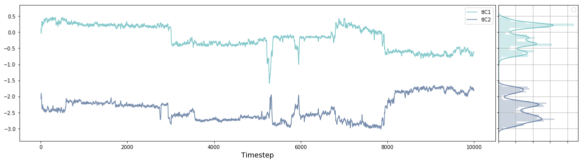
tICA is similar to principal component analysis (see "tICA vs. PCA" example). Note that the 84-dimensional space is reduced to 2 dimensions.
tica_model = tICA(lag_time=10, n_components=2, kinetic_mapping=True)
tica_trajs = tica_model.fit_transform(scaled_data)

ax, side_ax = msme.plot_trace(tica_trajs[0][:, 0], window=10,
                              label='tIC1', xlabel='Timestep')
_ = msme.plot_trace(tica_trajs[0][:, 1], window=10, label='tIC2',
                    xlabel='Timestep', color='rawdenim', ax=ax,
                    side_ax=side_ax)
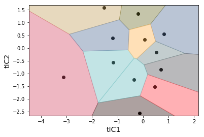
Conformations need to be clustered into states (sometimes written as microstates). We cluster based on the tICA projections to group conformations that interconvert rapidly. Note that we transform our trajectories from the 2-dimensional tICA space into a 1-dimensional cluster index.
clusterer = MiniBatchKMeans(n_clusters=12, random_state=rs)
clustered_trajs = clusterer.fit_transform(tica_trajs)

_ = msme.plot_voronoi(clusterer, xlabel='tIC1', ylabel='tIC2')
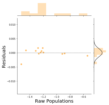
We can construct an MSM from the labeled trajectories and see how much it is perturbing the raw MD populations of a microstate.
In a large sampling regime, we should see a decorrelated cloud of points in the plot below. See this thread for a discussion on how to interpret this plot.
msm = MarkovStateModel(lag_time=1, n_timescales=5)
assigns = msm.fit_transform(clustered_trajs)

_ = msme.plot_pop_resids(msm, color='tarragon')
We can also plot the implied timescales. Remember that the timescales in the MarkovStateModel object are expressed in units of time-step between indices in the source data supplied to the fit() or fit_transform() methods.
_ = msme.plot_timescales(msm, ylabel=r'Relaxation Time (frames)')
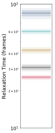
Those are the timescales of an MSM built at a lag time of 1 frame (for this dataset, each frame represents 50 ps).
Let's build several MSMs at lag times separated in log space to get a feel for when the MSM starts to have a Markovian behaviour.
msm_list = [
    MarkovStateModel(lag_time=x, n_timescales=5, verbose=False)
                     for x in [1, 10, 1e2, 1e3, 5e3, 9e3]
]

for msm in msm_list:
    msm.fit(clustered_trajs)
_ = msme.plot_implied_timescales(msm_list,
                                  xlabel=r'$\tau$ (frames)',
                                  ylabel='Relaxation Times (frames)')
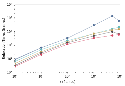
There is a tradeoff between the MSM accuracy and the fact that we have a limited amount of data. From the plot above we can see that using a lag time of around 1000 frames (or 50 ns) to build an MSM is appropriate (timescales have leveled off and there is a separation between the first and the second longest timescales).
We can inspect this timescales more closely now and express them in units of time:
msm = msm_list[3] # Choose the appropriate MSM from the list
for i, (ts, ts_u) in enumerate(zip(msm.timescales_, msm.uncertainty_timescales())):
    timescale_ns = ts * 50 / 1000
    uncertainty_ns = ts_u * 50 / 1000
    print('Timescale %d: %.2f ± %.2f ns' % ((i + 1), timescale_ns, uncertainty_ns))
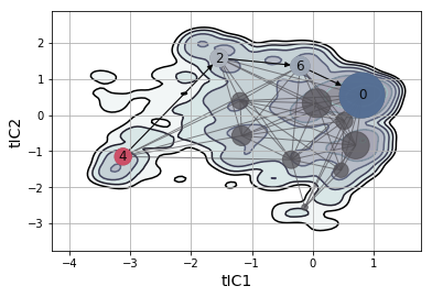
From our MSM and tICA data, we can construct a 2-D free energy landscape.
data = np.concatenate(tica_trajs, axis=0)
pi_0 = msm.populations_[np.concatenate(assigns, axis=0)]


# Free Energy Surface
ax = msme.plot_free_energy(data, obs=(0, 1), n_samples=10000,
                          pi=pi_0, gridsize=100, vmax=5.,
                          n_levels=8, cut=5, xlabel='tIC1',
                          ylabel='tIC2', random_state=rs)

# MSM Network
pos = dict(zip(range(clusterer.n_clusters), clusterer.cluster_centers_))
_ = msme.plot_msm_network(msm, pos=pos, node_color='carbon',
                          with_labels=False)


# Top Transition Pathway
w = (msm.left_eigenvectors_[:, 1] - msm.left_eigenvectors_[:, 1].min())
w /= w.max()
cmap = msme.utils.make_colormap(['rawdenim', 'lightgrey', 'pomegranate'])
_ = msme.plot_tpaths(msm, [4], [0], pos=pos, node_color=cmap(w),
                     alpha=.9, edge_color='black', ax=ax)
(Fs-Peptide-Example.ipynb; Fs-Peptide-Example.eval.ipynb; Fs-Peptide-Example.py)
